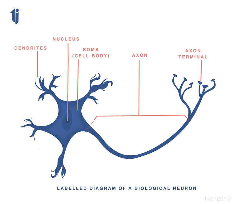
The functioning of biological neuron.
Dendrites extend from the neuron's cell body like branches of a tree extend from its trunk. However, in the human body, dendrites of one neuron connect to those of other neurons at a connection point called synapse.
Signal is received as inputs through the synapse which either excites(/fires/activates) the cell or inhibits its firing. The synaptic strength of each cell decides the intensity with which the cell fires up.
This product of input from the synapse into the synapse strength is summed up in the cell body. If this cummulative excitation, excedes the threshold value, the cell fires (or gets activated) and then further sends this signal down the axon to other neurons.
Biological neurons and their corresponding analogous artificial neurons
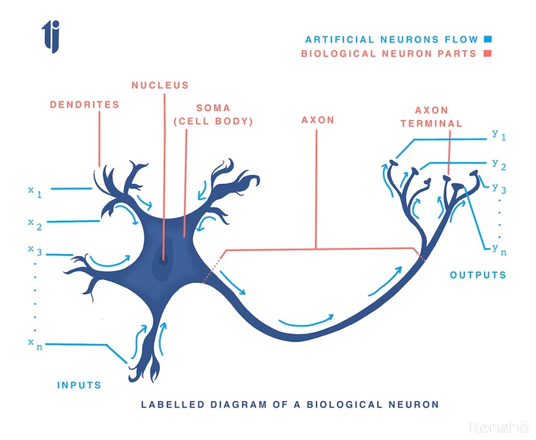
| Biological Neuron Parts | Analogous Artificial Neuron Parts or function |
|---|---|
| synapse via axon | source of input or destination of output |
| synaptic strength | weight (or strength) of each input for activation |
| cell body | Summation Block where cummulative frequency computed for resultant activation and compared to threshold |
The artificial neuron architecture
designed to mimic the first-order characteristics of biological neuron
A set of inputs are fed/applied of which, each input is also the representation of output of the neurons they come from. Each input is multiplied to its corresponding weight (synaptic strength) and then cummulatively summed up.
You can read The Importance of Synaptic Strength to understand its need via the real life applicability of sportsmanship.
Computational Layer
Summation Function or Summation Block
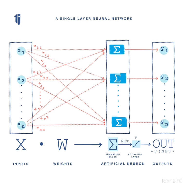
Let a set of inputs $x_{1}, x_{2}, ..., x_{n}$ be represented as a vector X, associated with a set of weight $w_{1}, w_{2}, ..., w_{n}$ represented as a vector W. Each input is multiplied to its corresponding weight, that is, each element of vector X is multiplied to each corresponding element in vector W. These products are cummulatively summed up (algebraically) in the summation block ( $∑$ ) producing an output called NET. The vector notation is hence follows:
$NET = XW$
Matrix Multiplication
The dimensions of matrix W are $m$ rows by $n$ columns, where $m$ is the number of inputs, and $n$ is the number of neurons. Hence, the weight connecting the third input to second neuron will be represented as $w_{3,2}$. Via simple matrix multiplication, NET and X are row vectors in $X \cdot W = NET$.
For illustration, let's take the example of the logical OR function.
| Input 1 | Input 2 | Output = Input 1 $\lor$ Input 2 |
|---|---|---|
| 0 | 0 | 0 |
| 0 | 1 | 1 |
| 1 | 0 | 1 |
| 1 | 1 | 1 |
This function can be represented in terms of matrices as follows where the two inputs, Input 1 and Input 2 are combined to form matrix $X$. A weight matrix is generated randomly of size 2x1 such that we get a resultant OUT matrix of dimension 4x1. Using the following operations we shall observe the output derived to approximate the values given in output above, regardless of the function used.
$$X \cdot W = NET$$$$ \begin{bmatrix} 0 & 0\\ 0 & 1\\ 1 & 0\\ 1 & 1 \end{bmatrix} \cdot \begin{bmatrix} 0.96231994\\ 0.53628568 \end{bmatrix} = \begin{bmatrix} 0\\ 0.53628568\\ 0.96231994\\ 1.49860562 \end{bmatrix}$$This can be implemented in python as:
import numpy

X = numpy.array([ [0,0],[0,1],[1,0],[1,1] ])

global w1
w1 = numpy.random.random((2,1))

numpy.dot(X,w1)
Activation Function or Processing Block
The output/signal received at NET is further process by an activation function F to produce the neuron's output signal, OUT. The activation functions checks like a biological neuron whether the signal must be fired up(or activated) or not. This can be represented as the following linear function: $OUT = K(NET)$, where $K =$ constant, threshold function. Hence,
$OUT = 1$ if $NET > T$
$OUT = 0$ otherwise
where $T$ is a constant threshold value, also known as bias.
Matrix
Checking the matrix output $NET$ and comparing it with threshold, $T$ as defined above taking $T = 0.5$:
$$T(NET) = OUTPUT$$$$T \begin{bmatrix} 0\\ 0.53628568\\ 0.96231994\\ 1.49860562 \end{bmatrix} = \begin{bmatrix} 0\\ 1\\ 1\\ 1 \end{bmatrix}$$Squashing Function
The processing block $F$ is called a squashing function when it compresses the range of $NET$ such that OUT doesn't exceed some low limits regardless of the value of NET.
Sigmoid
$F$ is often chosen to be the logistic function or "sigmoid" (which means S-shaped) represented mathematically as: $F(x) = 1/(1+e^{-x})$. Hence, $$OUT = 1/(1+e^{-NET})$$.
Activation function is a non-linear gain for the artificial neuron which is the ratio of the change in OUT to a small change in NET, also equal to the slope of the curve at a special excitation level.
| Excitation value | Shape of the curve | Activation function value |
|---|---|---|
| large, negative | ~ horizontal | low |
| zero | steep | high |
| large, positive | ~ horizontal | low |
Finding by Grossberg (1973)
The activation function's non linear gain characteristic solves the noise-saturation dilemma, "How can the same network handle both small and large signals?".
Hyperbolic Tangent
often used by biologists as a mathematical model of nerve-cell ativation
It is another commonly used activation function, expressed as:
$$\tanh(NET) = OUTPUT$$$$\tanh \begin{bmatrix} 0\\ 0.53628568\\ 0.96231994\\ 1.49860562 \end{bmatrix} = \begin{bmatrix} 0\\ 0.49017122\\ 0.7453099\\ 0.90489596 \end{bmatrix} \longrightarrow \begin{bmatrix} 0\\ 1\\ 1\\ 1 \end{bmatrix}$$Difference between the Sigmoid Logistic function and Hyperbolic Tangent function
| Sigmoid Logistic function | Hyperbolic Tangent function | |
|---|---|---|
| Mathematical Function | $OUT = 1/(1+e^{-NET})$ | $OUT = \tanh(NET)$ |
| Shape | S-shaped, throughout positive | S-shaped, symmetrical about origin |
| Condition for OUT = 0 | NET ≤ T | NET = 0 |
| Values for OUT | Positive (Unipolar) | Bipolar |
Limitations with respect to biological counterpart
- It overlooks the time delays affecting the system dynamics, rather inputs produce immediate outputs.
- It overlooks the synchronism or the frequency-modulation of the biological neuron.
Single Layer Artificial Neural Networks
The number of layers in an artificial neural network is determined by the number of computational layers in the network, that is, the layers that process the NET to produce OUT. The circular nodes on the left-most only distribute the inputs and perform no computation hence, will not considered to constitute a layer.
The set of inputs X has each of its elements connected to each artificial neuron through a separate weight.
Multi Layer Artificial Neural Networks
Multilayer networks may be formed by cascading a group of single layers as the output of one layer provides the input to the subsequent layers. Though this would not provide any increase in computational power unless there is a non-linear activation function between layers.
This can be expressed with vectors as:
If there is no non-linear activation function in between layers, the output from the product of input and the intial weight layer will serve as the input to be multiplied with the next weight layer, that is: $$(XW_{1})W_{2}$$ Since matrix multiplication is associative: $$= X(W_{1}W_{2})$$
Hence, a two layer linear network is equivalent to a single layer linear network having a weight matrix equal to the product of the two weight matrices.
Python Code Implementation
Single Layer Neural Network
import numpy
#input layer
X = numpy.array([ [0,0],[0,1],[1,0],[1,1] ])

#expected output layer
y = numpy.array([[0,1,1,1]]).T

#weight matrix
global w1
w1 = numpy.random.random((2,1))

dot_product = numpy.dot(X,w1)

print("X = ",)
print(X)
print("")
print("y = ",)
print(y)
print("")
print("weight matrix w1 = ",)
print(w1)
print("-"*60)
print("dot product of x and w1 = ",)
print(dot_product)
def threshold_value(x, threshold=0.5):
    OUT = numpy.empty( [ len(x),len(x[0]) ] )
    for m in range(len(x)):
        for n in range(len(x[0])):
            if x[m][n] > threshold:
                OUT[m][n] = 1
            else:
                OUT[m][n] = 0
    return OUT

def sigmoid(x, derivative = False):
    if derivative == True: return x(1-x)
    return (1/(1 + numpy.exp(-x)))

def tanh(x):
    return numpy.tanh(x)

def compute_single_layer(summation, activation='sigmoid'):
    if activation == 'threshold_value':
        layer1 = threshold_value(summation)
    elif activation == 'sigmoid':
        layer1 = sigmoid(summation)
    elif activation == 'tanh':
        layer1 = tanh(summation)
    return layer1
print("-"*60)
print("Output with threshold value activation = ",)
print(compute_single_layer(dot_product,'threshold_value'))
print("-"*60)
print("Output with sigmoid activation = ",)
print(compute_single_layer(dot_product,'sigmoid'))
print("-"*60)
print("Output with tanh activation = ",)
print(compute_single_layer(dot_product,'tanh'))
Multi Layer Neural Network
#input layer
X = numpy.array([ [0,0],[0,1],[1,0],[1,1] ])

#expected output layer
y = numpy.array([[0,1,1,1]]).T

#weight matrix
global w01
w01 = numpy.random.random((2,3))

global w02
w02 = numpy.random.random((3,1))

print("X = ",)
print(X)
print("")
print("y = ",)
print(y)
print("")
print("weight matrix w1 = ",)
print(w01)
print("")
print("weight matrix w2 = ",)
print(w02)
Computing (x . w01 ) . w02
layer_1 = numpy.dot(X, w01)
layer_2 = numpy.dot(layer_1, w02)
print("(x . w01 ) . w02 = ",)
print(layer_2)
Computing x . (w01 . w02)
layer_1 = numpy.dot(w01, w02)
layer_2 = numpy.dot(X, layer_1)
print("x . (w01 . w02) = ",)
print(layer_2)
Hence, proved that (x . w01 ) . w02 = x . (w01 . w02)
This implies that the number of layers in a neural network is defined by number of computational layers (those using non-linear activation functions).
References
[1] P. D. Wasserman, Neural computing: theory and practice. Estados Unidos: Van Nostrand Reinhold, 1989.